This demo helps students visualize the time dependent behaviors exhibited by a capacitor with an AC input. It shows that when charging a capacitor, in series with a resistor, the capacitor voltage will depend on the time constant

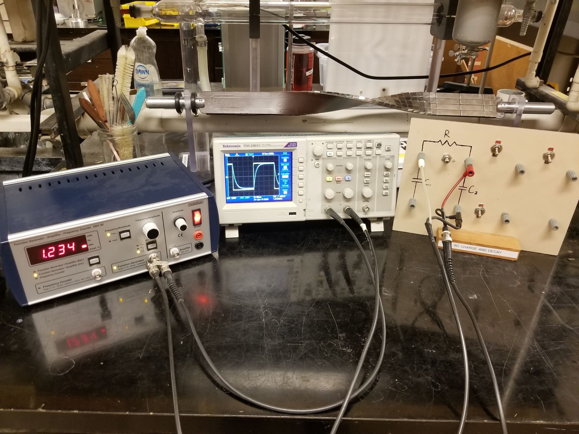
Figure 1: RC Charge and Discharge Setup
Materials:
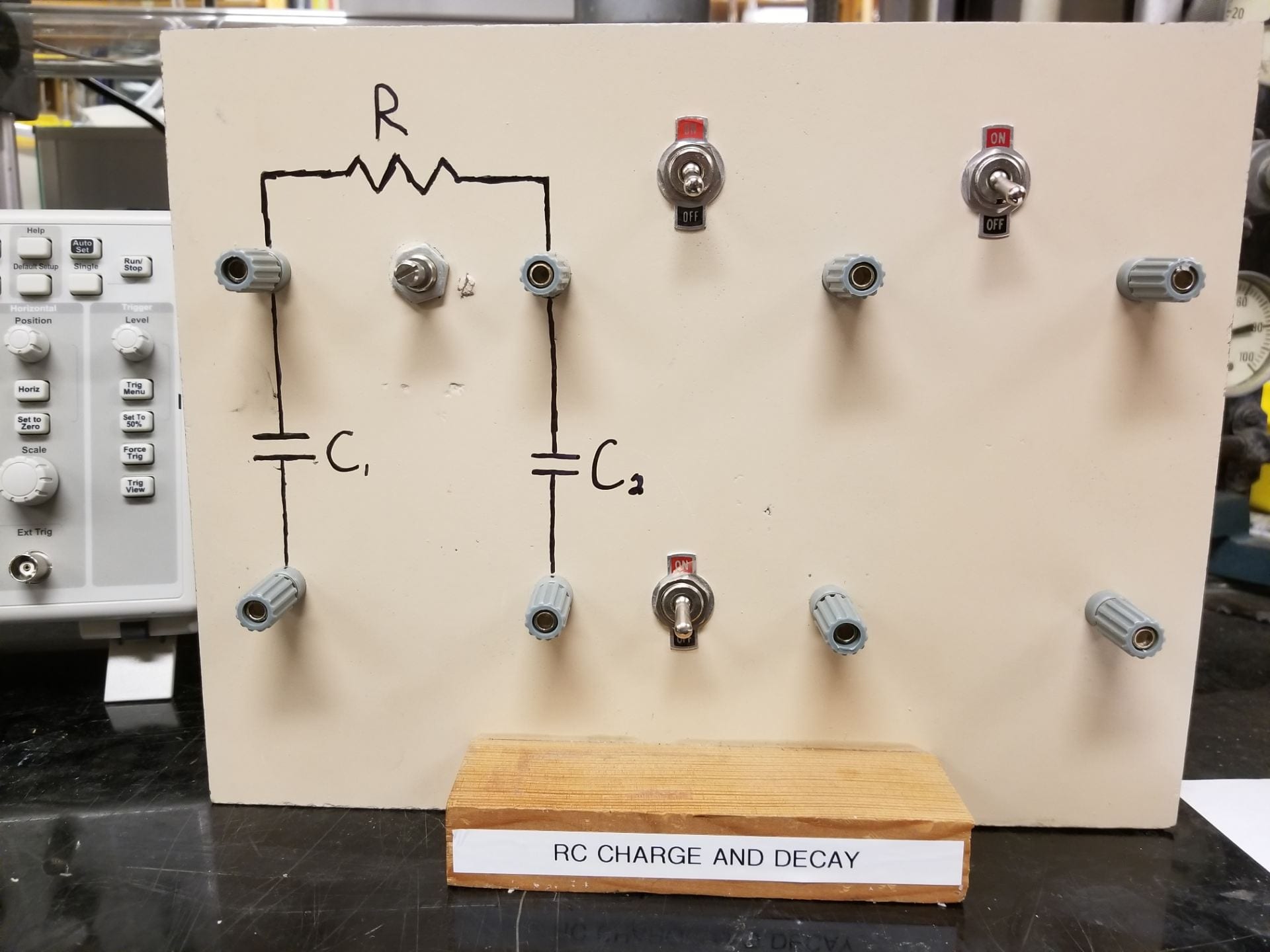
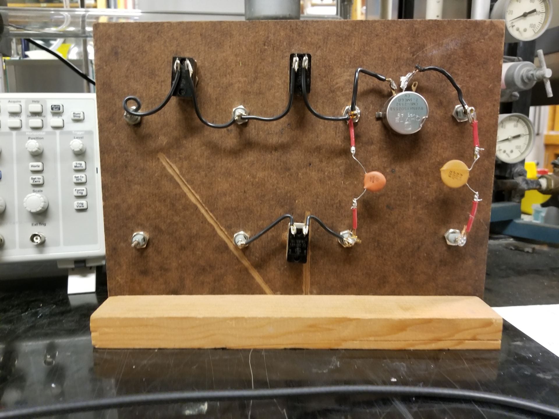
- RC board: This board has a variable resistor two capacitors attached to the back, and allows for a variety of connections between the three (Figure 2). The variable resistor, or potentiometer, allows for adjustments of the time constant which affects how quickly the capacitor charges and discharges. In this setup we will only use
and
, the orange capacitor in (Figure 3).

Figure 2: RC Board

Figure 3: Back Side of the RC Board
- Function Generator: Produces an AC voltage to charge and discharge the capacitor. (Figure 4)

Figure 4: AC Function Generator
- Oscilloscope: Helps visualize the behavior of the output voltage as a function of time, and is compared with the input voltage from the function generator. Figure 5 below shows the ideal scope image for a full charge and full discharge. (Figure 5)
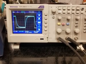
Figure 5: Oscilloscope
- BNC Cables: Three BNC cables are required to make connections between the function generator to RC board, function generator to oscilloscope, and oscilloscope to RC board. One must be BNC to BNC while the other two are BNC cables with male banana jack ends.


Setup:
For the RC charge and decay setup we will only need the potentiometer
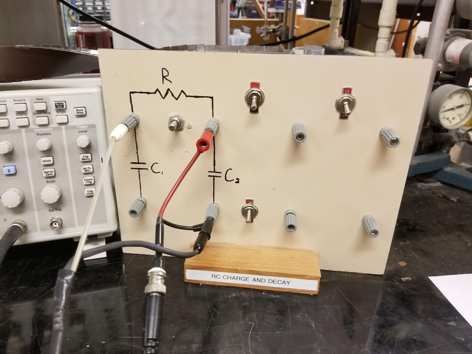
Figure 6: RC Charge and Discharge Setup
For reference, the white and black banana jacks come from the function generator to supply the input voltage. They connect the resistor and capacitor in series. The red and black banana jacks come from the oscilloscope to measure the output voltage, where the output voltage is taken across the capacitor. The circuit diagram for this setup can be seen below in Figure 7.
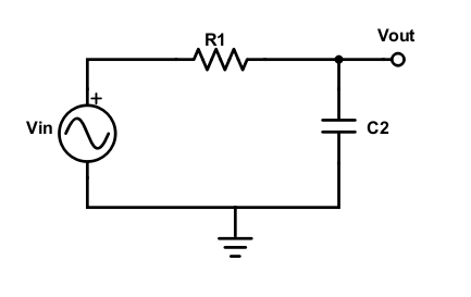
Figure 7: Circuit Diagram for RC Charge and Decay
This demo works for a wide range of frequencies set on the function generator, so this setting doesn’t need to be precise. In order to avoid non-ideal effects from the function generator it’s best to stay at least above 500 Hz. A simple way to tune the charge and discharge is to set the frequency around 10 kHz, then vary the potentiometer. This is the knob located below the R drawn on the RC board. Turning this knob either clockwise or counterclockwise will adjust the resistance, which will in turn alter the time constant dictating the charge and discharge time of the capacitor. These adjustments allow for an oscilloscope image similar to that of Figure 5. It needn’t be exactly like this, but it gives a more complete picture of the behavior to have one full charge and one full discharge visible on the screen. It will likely also be necessary to adjust the settings on the oscilloscope. This can be done using auto set or adjusting manually.
The black auto set button can be found in the top right corner of the oscilloscope. It provides a reasonable view. Alternatively, the image may be adjusted manually using the three knobs in a row seen in Figure 5. The leftmost adjusts amplitude (y scaling) of channel one, the center adjusts amplitude of channel two, and the rightmost knob adjust the time scale (x axis/scaling) of both channels. There is also a black auto set button in the top right corner of the oscilloscope which provides a reasonable view.
Explanation:
To show why the capacitor voltage has this unusual exponential dependence on time, and why the time constant depends on both R and C we begin with the circuit diagram in Figure 7. From this and Kirchhoff’s junction rule that the current flowing through each element is equal.

We can also see that by Kirchhoff’s loop rule the voltage rise caused by the input must be equal to that dropped over the resistor and capacitor.

From here we can use Ohm’s law, the definition of current through a capacitor, and a little calculus to get to our final result.

R + V_c \:\: using \:\: I_c=I_r \:\: and \:\: I_c=C\cfrac{dV_c}{dt}")


![\left[ln(V_{in} - V'_c)\right]^{V_c}_0 = \cfrac{1}{RC}[t']^{t}_{0}](https://s0.wp.com/latex.php?latex=%5Cleft%5Bln%28V_%7Bin%7D+-+V%27_c%29%5Cright%5D%5E%7BV_c%7D_0+%3D+%5Ccfrac%7B1%7D%7BRC%7D%5Bt%27%5D%5E%7Bt%7D_%7B0%7D&bg=ffffff&fg=000000&s=0 "\left[ln(V_{in} - V'_c)\right]^{V_c}_0 = \cfrac{1}{RC}[t']^{t}_{0}")
 + ln(V_{in}) = \cfrac{t}{RC}")
 = - \cfrac{t}{RC}")
![exp[\cfrac{-t}{RC}] = \cfrac{V_{in} - V_c}{V_{in}}](https://s0.wp.com/latex.php?latex=exp%5B%5Ccfrac%7B-t%7D%7BRC%7D%5D+%3D+%5Ccfrac%7BV_%7Bin%7D+-+V_c%7D%7BV_%7Bin%7D%7D&bg=ffffff&fg=000000&s=0 "exp[\cfrac{-t}{RC}] = \cfrac{V_{in} - V_c}{V_{in}}")
![exp[\cfrac{-t}{RC}] = 1 - \cfrac{V_c}{V_{in}}](https://s0.wp.com/latex.php?latex=exp%5B%5Ccfrac%7B-t%7D%7BRC%7D%5D+%3D+1+-+%5Ccfrac%7BV_c%7D%7BV_%7Bin%7D%7D&bg=ffffff&fg=000000&s=0 "exp[\cfrac{-t}{RC}] = 1 - \cfrac{V_c}{V_{in}}")
![\cfrac{V_c}{V_{in}} = 1 - exp[\cfrac{-t}{RC}]](https://s0.wp.com/latex.php?latex=%5Ccfrac%7BV_c%7D%7BV_%7Bin%7D%7D+%3D+1+-+exp%5B%5Ccfrac%7B-t%7D%7BRC%7D%5D&bg=ffffff&fg=000000&s=0 "\cfrac{V_c}{V_{in}} = 1 - exp[\cfrac{-t}{RC}]")
![V_c= V_{in}(1 - exp[\cfrac{-t}{RC}])](https://s0.wp.com/latex.php?latex=V_c%3D+V_%7Bin%7D%281+-+exp%5B%5Ccfrac%7B-t%7D%7BRC%7D%5D%29&bg=ffffff&fg=000000&s=0 "V_c= V_{in}(1 - exp[\cfrac{-t}{RC}])")
![V_c= V_{in}(1 - exp[\cfrac{-t}{\tau}])](https://s0.wp.com/latex.php?latex=V_c%3D+V_%7Bin%7D%281+-+exp%5B%5Ccfrac%7B-t%7D%7B%5Ctau%7D%5D%29&bg=ffffff&fg=000000&s=0 "V_c= V_{in}(1 - exp[\cfrac{-t}{\tau}])")
where 
From these calculations we can see where the time constant 


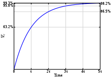
Figure 8: RC charge curve from Wikipedia
The figure above depicts a capacitor as it is charged, showing the behavior of the function we derived above. We can see that at
Written by: Noah Peake