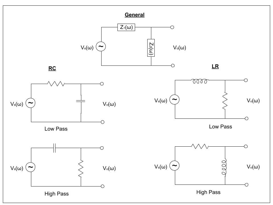
Figure 1: The general circuit diagram used for calculations. The low and high-pass versions of the RL and RC circuits can be seen on the right and left, respectively. Vs(w) is the voltage of the function generator and Vo(w) is the voltage on the oscilloscope.
This demo is designed for students who have already learned the basics of RC and RL circuits. Through this demo, students can see one of the applications: simple low-pass and high-pass filters. Students will be able to understand how the arrangements of resistive, capacitive, and inductive loads can produce opposite effects.
Materials:
- RC filter board: This board has a variable resistor and capacitor attached to the back, and allows for a variety of connections between the two (Figure 2). The variable resistor, or potentiometer, allows for adjustments of the cutoff frequency of the filters. (Figure 3)
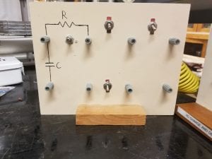
Figure 2: RC board
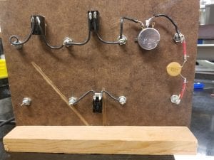
Figure 3: RC Board Wiring
- Function Generator: Produces an AC voltage to excite the RC filters. (Figure 4)

Figure 4: AC Function Generator
- Oscilloscope: Helps visualize the behavior of the output voltage as a function of time, and is compared with the input voltage from the function generator. (Figure 5)
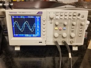
Figure 5: Oscilloscope
- BNC Cables: Three of the BNC cables are required to make connections between the function generator to RC board, function generator to oscilloscope, and oscilloscope to RC board. One must be BNC to BNC while the other two are BNC cables with male banana jack ends.


Setup:
The RC board (Figure 2) facilitates both an RC low-pass and RC high-pass filters. To change between these two setups, one only needs to change the input and output voltage banana jack cable positions. Figure 6 below shows the banana jacks plugged into the board in a low-pass configuration. The diagram for this circuit can be seen above in Figure 1, in the mid-left schematic.
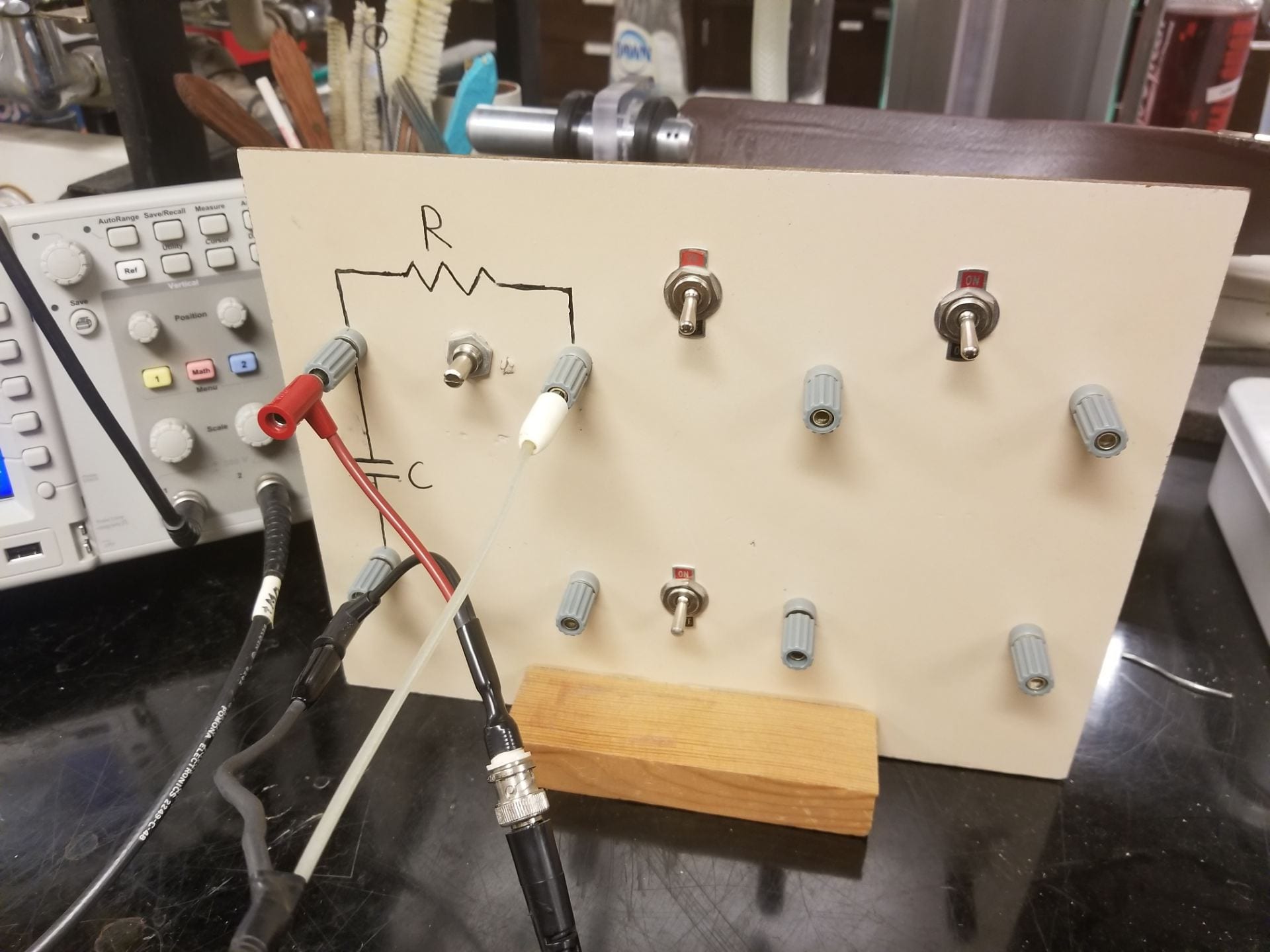
Figure 6: Low-pass Configuration
This low-pass configuration is characterized by being grounded on the open node of the capacitor. Both black banana jacks should attach to the capacitor’s open end. As for the red and white jacks, the red jack should attach to the shared node between the resistor and capacitor, while the white jack should attach to the resistor’s open node.The white jack is on the other end of the BNC cable attached to the function generator and the red jack is on the other end of the BNC attached to the oscilloscope. The color isn’t important, so long as the oscilloscope measures the output voltage across the capacitor, and the function generator is supplying an input voltage to the resistor’s open node. This configuration can be seen in circuit diagram form in either Figure 1 above or in Figure 10 below.
The board layout can be seen below in Figure 7 for the RC high-pass configuration. The circuit diagram is above in Figure 1 in the bottom left corner.
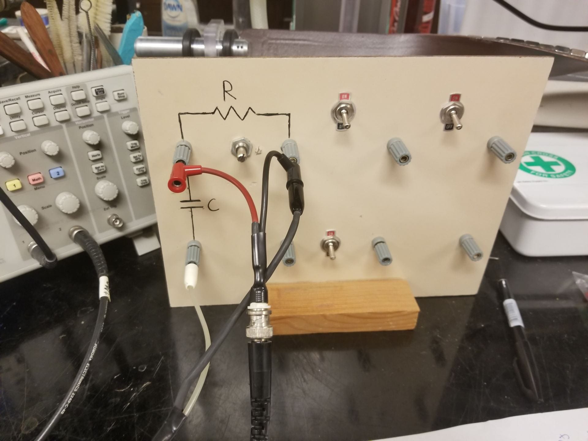
Figure 7: High-pass Configuration
The notable difference between these two layouts being that both grounds have switched positions with the white jack. The output voltage will now be measured across the resistor. More explicitly, the resistor’s open node should be grounded, while the capacitor’s open node has the white jack attached to supply the input voltage. The output voltage is still taken from the shared node, but in this case it measures the output voltage across the resistor as opposed to the capacitor as in the low-pass filter.
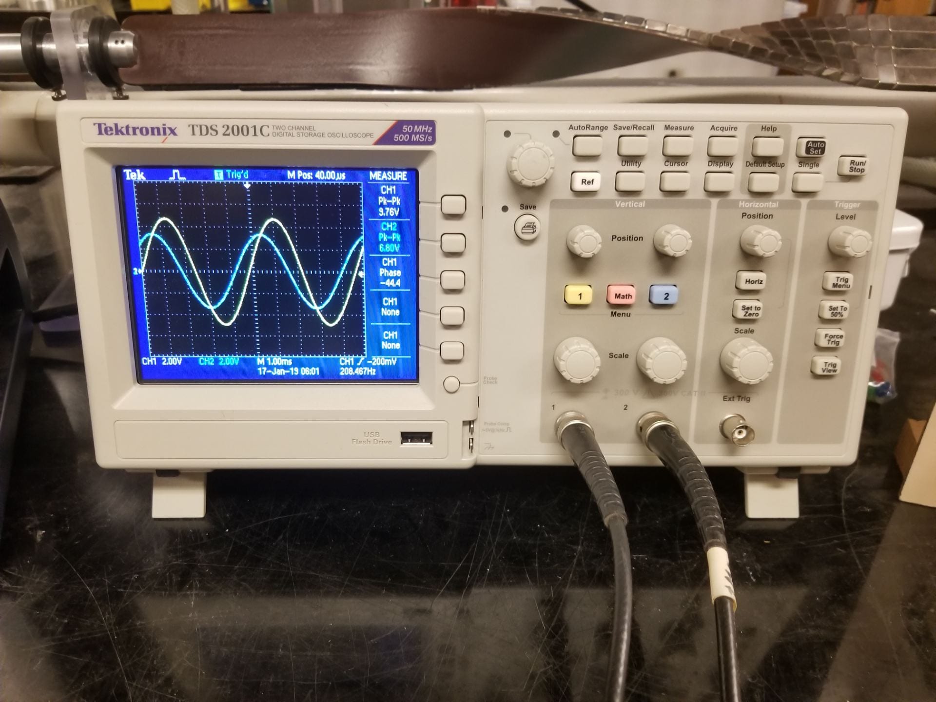
Once all the connections are made, one can now sweep through the frequencies to observe the attenuation (decrease of the output compared to the input) above or below the cutoff frequency. To start, set the function generator to produce a sine wave of about 500 Hz. Next, push measure on the oscilloscope to compare the input (Ch 1) and output (Ch 2) voltages. Now vary the potentiometer (turnable dial on the RC board) until the output is about .7 times the input voltage. To do this, set the input voltage to a round number such as 10 or 1 volts, making the desired output voltage 7 and .7 volts respectively. By varying the resistance, we are setting the critical frequency to 500 Hz. Once this is set up, sweeping the frequency higher or lower on the function generator will take you above or below the cutoff frequency, either increasing or decreasing the attenuation of the signal. With the high-pass filter, increasing the frequency will slightly raise the output, while decreasing the frequency will drastically decrease the output. The low-pass will experience an output drop upon increasing the frequency, and a slight increase in output if the frequency is decreased. The goal of this stage can be seen in Figure 8 below.
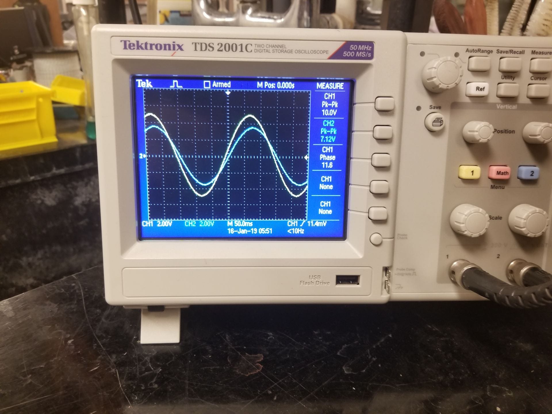
Figure 8: The Elusive Cutoff Frequency
Explanation:
The simple explanation for the RC high-pass and low-pass begins with understanding how capacitors react to alternating current, and observing extreme cases. The current allowed through a capacitor is equal to its capacitance multiplied by the time derivative of its voltage. =C* \cfrac{dV_c}{dt}")

Figure 9: RC High-Pass Circuit Diagram, courtesy of the Electronics Tutorials website
In the diagram above in Figure 9, we can see that as the frequency approaches zero, the input current will be blocked by the capacitor. This tells us that the as the frequency decreases, current to the resistor will be limited. This will limit the resistor’s current, decreasing the output voltage. As frequency increases, the capacitor increasingly acts like a short. This allows more and more current to pass from the input through the resistor, causing a higher output voltage.
We can also make this argument mathematically based on the impedances of a capacitor and resistor. Impedance refers to the complex number analogue of resistance. For the high-pass filter derivation we refer to the components of the circuit diagram in Figure 9 above.
We start with 

We can use Ohm’s Law to find a relation for the input and output voltages.
 = (Z_c + Z_r)*I(\omega)")
 = I(\omega)*Z_r")
For the high-pass filter, we can combine the two equations above to find the output voltage as a function of frequency.
 = V_i(\omega)*(\cfrac{Z_r}{Z_r+Z_c}) = V_i(\omega)*(\cfrac{j\omega RC}{1+j\omega RC})")
From this we can see that:
As 
\rightarrow V_i(\omega)")
And as 
\rightarrow0")
We can construct a similar argument for the low-pass filter shown below in Figure 10.

Figure 10: RC Low-Pass Circuit Diagram, courtesy of the Electronics Tutorials website
We can use the same arguments as above to understand the extreme behavior of this filter. When frequency decreases near zero, the capacitor acts like an open circuit, blocking most current from passing. By blocking most current from grounding through the capacitor, it forces the signal to pass to the output. This results in a large output voltage for lower frequencies. As frequency increases towards infinity the capacitor begins to act like a short, allowing all current provided by the input to ground through the capacitor. By allowing current to flow through the capacitor with little resistance the capacitor ensures higher frequency signals won’t be received at the output.
From the high-pass derivation we can use the same impedances and Ohm’s Law equation. However, our output voltage has changed slightly because it is now taken across the capacitor.
 = I(\omega)*Z_c")
Using a similar set of equations as used for the high-pass, we derive the final frequency dependent output voltage equation.
 = V_i(\omega)*(\cfrac{Z_c}{Z_r+Z_c}) = V_i(\omega)*(\cfrac{1}{1+j\omega RC})")
From this we can see that:
As
And as
To determine the middle ground between these two extremes we define the cutoff frequency as shown below.
Cutoff Frequency:

or 

An important note is that this equation holds for both high-pass and low-pass RC filters with the same resistor and capacitor. For a low-pass filter, increasing past the cutoff frequency will cause the output amplitude to drop. As for the high-pass filter, decreasing the frequency below the cutoff will cause a similar decrease in output voltage. This frequency divides the region of signals passed and signals attenuated at the output.
One might also be curious as to how quickly each of these output voltages drop off as frequency changes. To understand this, a plot sweeping frequency versus gain is most effective. Gain refers to the log of the ratio of output voltage to the input voltage: ")
One important example of gain is -3 dB. For reference, a gain of -3 dB equates to a ratio of 

With this information in mind, we can now make sense of a plot of output versus frequency for high-pass and low-pass filters. Below are two such plots, one for high-pass (Figure 11) and one for low-pass(Figure 12).

Figure 11: High-Pass RC Filter Frequency Sweep, provided by the Electronics Tutorials website

Figure 12: Low-Pass RC Filter Frequency Sweep, provided by the Electronics Tutorials website
These graphs help us visualize how each of the RC filters we’ve discussed will respond given a wide range of frequencies. To clarify some terms used in these graphs, pass band refers to the frequency range in which an input AC signal is allowed to pass to the output, while stop band refers to the frequency in which the input is stopped or blocked. The 
The plots verify the previous calculations done for extreme cases, but also fill in areas we were unable to quantify with rudimentary limit analysis. An important concept to grasp is that when performing the RC filter demo described above, the audience will be shown a single point on these graphs. The frequency will be set to one particular value, and the oscilloscope will show the input and output alternating voltages of the filter. In order to visualize this behavior, one must sweep through the frequencies and observe the resulting output amplitudes. The output versus input voltages will follow these plots, rising or falling depending where one is on the curve. The best region to sample will be around the cutoff frequency or 3 dB point which is at the cutoff frequency.
Separating the concept of output versus time, as shown by the oscilloscope, and output versus frequency, as shown by the plots above, is a difficult but necessary process for solid understanding. Frequency plots show us an overall trend the filter follows, describing its general characteristics. A time plot shows us one snapshot of the frequency plot. With the frequency held constant we observe variations of the output amplitude over the span of some time.
Written by: Noah Peake