Magnetically Coupled Harmonic Oscillators | UCSC Physics Demonstration Room

Figure 1.

Figure 2

Materials

Two large inductor coils (solenoids) – F4
Two identical springs – C3
Two weight hooks with circular base – A3
10 small square magnets (split to make two bar magnets) – F3
50 mV Voltmeter – F3
Oscilloscope – K1
Banana to BNC converter
Two bench stands with talon attachments
2x Banana cables

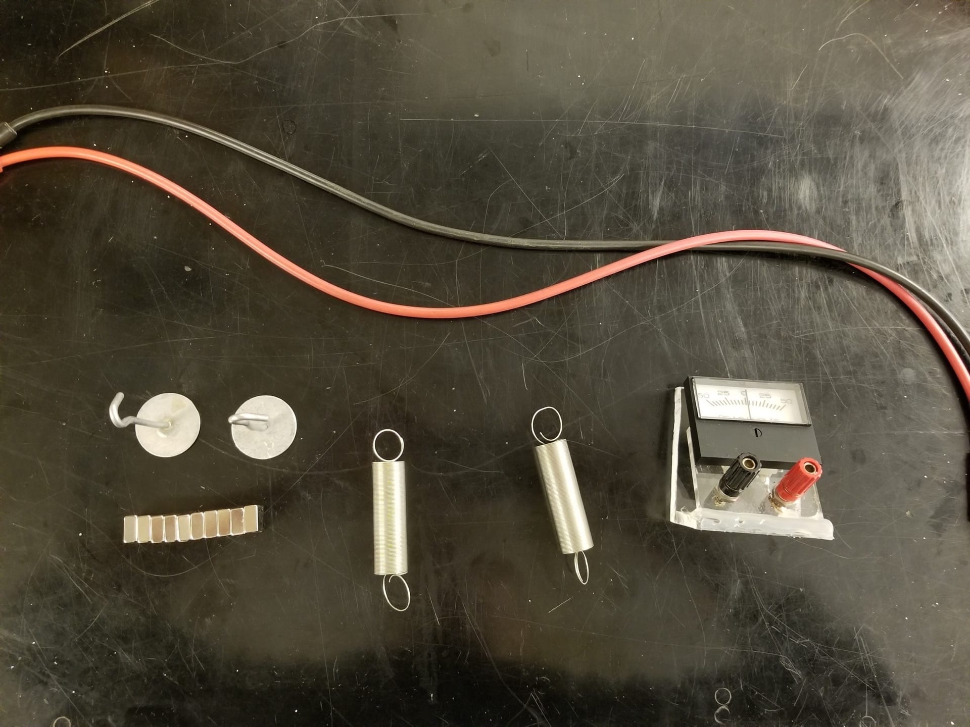
Figure 3. Solenoid, stands & talon clips not pictured.

Demonstration

Version 1:
This version of the demo is consisted of single magnet on a spring oscillating inside a solenoid. This demonstrates the relationship between current and magnetic fields. It also shows energy conservation in mechanical and electromagnetic systems.

To set up this demonstration, attach the talon clips to the bench stand and hang the spring from it (tape can be used to hold the spring in place). Attach one square magnet to the top of its base, and the rest to the bottom. Then hang the magnets from the spring. Place the solenoid as seen in Fig 2. Attach the banana cables from the solenoid directly to the voltmeter.
When the magnets are displaced, the spring will oscillate, dipping the magnets in and out of the solenoid. The change in magnetic field causes a current in the solenoid, visible on the voltmeter.

In place of the voltmeter, an oscilloscope allows students to view the time-varying nature of the induced voltage in the inductor. To set up this version, attach a BNC to banana jack converter to channel 1 on the oscilloscope. Then attach the same leads that hooked into the voltmeter instead into the oscilloscope. With these connections made, use a time scale of 250 miliseconds and a voltage scale of 100 miliVolts to best view the changing voltage of the inductor. An example of what the oscilloscope screen should look like is shown in Figure 4 below. If the sine wave has peaks of alternating maximums, then adjust the clamp holding the spring such that the mass freely hangs in the direct center of the solenoid vertically.

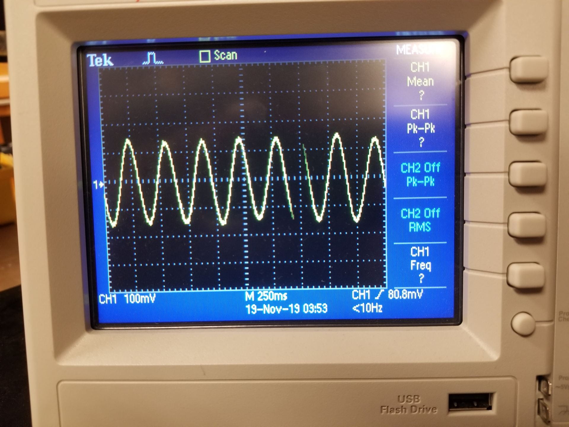
Figure 4: Oscilloscope view of inductor voltage

Version 2:

The second version of this demonstration is to show the nature of coupled oscillators whose energy transfer is mediated by a magnetic field. It consists of two identical springs and magnets oscillating in two identical solenoids which are connected in series with each other. The coupling of these mechanical oscillators is electromagnetic and due to the oscillating currents flowing between the solenoids.

To set up this demo, repeat and reflect the previous set up. This time, attach two solenoids in series without the voltmeter. Now, when mass one is displaced and mass two is still, the other will start oscillating in or out of phase with the original mass; depending on orientation of the solenoids.

Explanation:

Figure 5. Diagram of a moving conducting loop of wire in a non-uniform magnetic field. We will use these same variables for our analysis.

We will begin by analyzing version one, but as a first step we will consider the interaction force between a single-turn of the coil. Namely, N=1.
In Figure 5, a conducting ring moves at velocity v upwards. Since the magnetic field (denoted by B) is non-linear, this causes a changing flux Φ through the ring which in turn induces an emf given by:

$\varepsilon_i = \oint (v \times B) \,dl$
$= 2\pi avB_\rho$

If μ is the magnets intrinsic dipole moment, then we can use a magnetic dipole approximation for B_ρ

$B_\rho = \frac{3\mu za}{(a^2 + z^2)^{5/2}}$

The magnetic force on the ring is then given by the relation

$F = \int I \times B \,dl$
$= 2\pi aB_{\rho} \frac{\varepsilon_i}{R}$
$= \frac{(2\pi aB_\rho)^2v}{R}$

Thus,

$F = \frac{(6 \pi \mu za^2)^2 v)}{(a^2 + z^2)^{5/2}R}$

Where,

$R = \frac{L}{\sigma A}$
$R = \frac{2 \pi a}{\sigma (\pi r^2)}$

This is therefore the magnetic force on a single coil of wire. To expand as an N-turn coil of length L, recall that the number of turns in an element of coil dz is

$dN = \frac{N}{L} dz$

Now integrating the first equation over N gives,

$\varepsilon_i = \int_{d}^{d+L} 2 \pi avB_\rho \frac{N}{L} dz$
$\varepsilon_i = \frac{6\pi N a^2\mu v}{L} \int_{d}^{d+L} \frac{z}{(a^2 + z^2)^{5/2}} dz$
$\varepsilon_i = \frac{2\pi N a^2\mu v}{L} \frac{-1}{(a^2+z^2)^{3/2}}$

Where d is the displacement from the spring’s equilibrium point to the top of the coil. This equation evaluated produces the following,

$\varepsilon_i = 2\pi a^2\mu v \frac{N}{L}[\frac{1}{(a^2 +d^2)^{3/2}} - \frac{1}{(a^2 +(d+L)^2)^{3/2}}],$

Thus by the same process as previously, the total magnetic force on the entire coil is:

$F = (2\pi a^2\mu\frac{N}{L})^2 \frac{v}{R}[\frac{1}{(a^2 +d^2)^{3/2}} - \frac{1}{(a^2 +(d+L)^2)^{3/2}}]^2 ,$

Figure 6. Diagram showing the two springs and magnets oscillating about each coil.

Now that we have the force on the entire coil of wire, the next step is to analyze the equations of motion for two equal oscillating magnets.

As seen in Figure 6, the elongation variables are x₁(t) & x₂(t) of each spring, respectively. The distances from each coil to the equilibrium point of the springs are b, respectively.

Figure 7. Diagram modeling the simple circuitry of the induced emfs and resistances

Electrically, we can imagine that this apparatus forms a simple series circuit with two (hopefully equal) resistors and two voltage sources, as shown in Figure 7. As we can see in Figure 6, d now can be expanded as d = b – x, respectively. Thus, we can use our equation for the emf derived above as:

$\varepsilon_1 = 2\pi a^2\mu \dot{x_1} \frac{N}{L}[\frac{1}{(a^2 +(b_1 - x_1)^2)^{3/2}} - \frac{1}{(a^2 +(b_1 - x_1 + L)^2)^{3/2}}],$

Where we have an analogous expression for the emf generated in the second coil; in terms of x₂(t) and b₂. respectively.

Now we can use Kirchoff’s Laws and Figure 6 to get the following:

$I(t) = \frac{\varepsilon_1 -\varepsilon_2}{R_1 + R_2}$

Substituting in the respective emf terms and solving gives:

$I_i(t) = \frac{N}{L}(2\pi a^2 \mu) [\frac{1}{(a^2 +d^2)^{3/2}} - \frac{1}{(a^2 +(d+L)^2)^{3/2}}] \frac{\dot{x_1} - \dot{x_2}}{R_1+R_2}$

Under the assumptions that $x_i(t) << b_i, x_i(t) << a_i$ and equal set up positions, that is, $b_i = b$ . Alongside the assumptions we made earlier of equal magnets, springs and solenoids.

As shown before, this gives an opposing magnetic force of:

$F = [\frac{N}{L}(2\pi a^2 \mu)]^2 [\frac{1}{(a^2 +d^2)^{3/2}} - \frac{1}{(a^2 +(d+L)^2)^{3/2}}]^2 [\frac{\dot{x_1} - \dot{x_2}}{R_1+R_2}]$

Finally, we want to find the oscillators’ equations of motion. We do this using the Newton’s Second Law! However, first let’s call C (units of 1/s) the entire constant in the above equation. Namely,

$C = \frac{1}{R_1+R_2}[\frac{N}{L}(2\pi a^2 \mu)]^2 [\frac{1}{(a^2 +d^2)^{3/2}} - \frac{1}{(a^2 +(d+L)^2)^{3/2}}]^2$

Such that,

$F = mC (\dot{x_1} - \dot{x_2})$

Now we can apply Newton’s Second Law,

$m\ddot{x_1} = -k_1 x_1 - mC (\dot{x_1} - \dot{x_2})$

Finally giving

$\ddot{x_1} + C\dot{x_1} + \omega_0^2 x_1 = C\dot{x_2}$
$\ddot{x_2} + C\dot{x_2} + \omega_0^2 x_2 = C\dot{x_1}$

Where the oscillators’ natural frequency is given by $\omega_0^2 = \frac{k}{m}$ , holding to our assumptions that k and m are equal for both oscillators. These equations then represent the two coupled equations of motion for the electromagnetically driven damped harmonic oscillators.

Notes

Written by Phoenix Gallagher

Edited by Noah Peake (oscilloscope section)