Double Atwood Machine | UCSC Physics Demonstration Room

Equipment:

2 single pulleys
Waxed string (this helps prevent the string from slipping of the pulley)
3 masses of varying weights (these should fall within the range (~200g-1kg)
Pegboard

Demo:

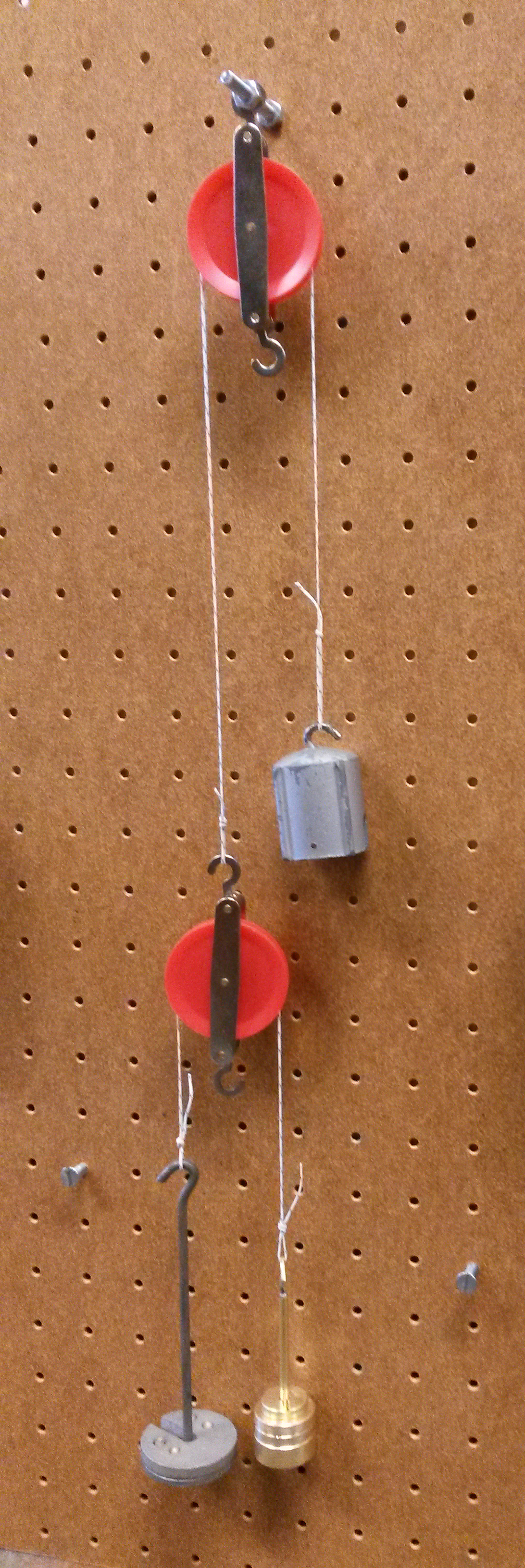
The double Atwood machine is a natural extension to the commonly used Atwood machine. Consisting of a string draped over a pulley with a mass on one end, this version of the classic demonstration has a second pulley attached to the other end of the string. This secondary pulley then has a second string draped over it with masses attached to the opposite ends of the string. The setup is depicted in Figure 1.

Figure 1: Demo for Double Atwood machine.

Explanation:

The double Atwood machine is commonly used to demonstrate the effects of classical mechanics, while introducing students to the mathematical concepts of Lagrange. The Lagrangian method makes finding the equations of motion for the masses much simpler than using Newton’s second law to determine the forces acting on each mass.

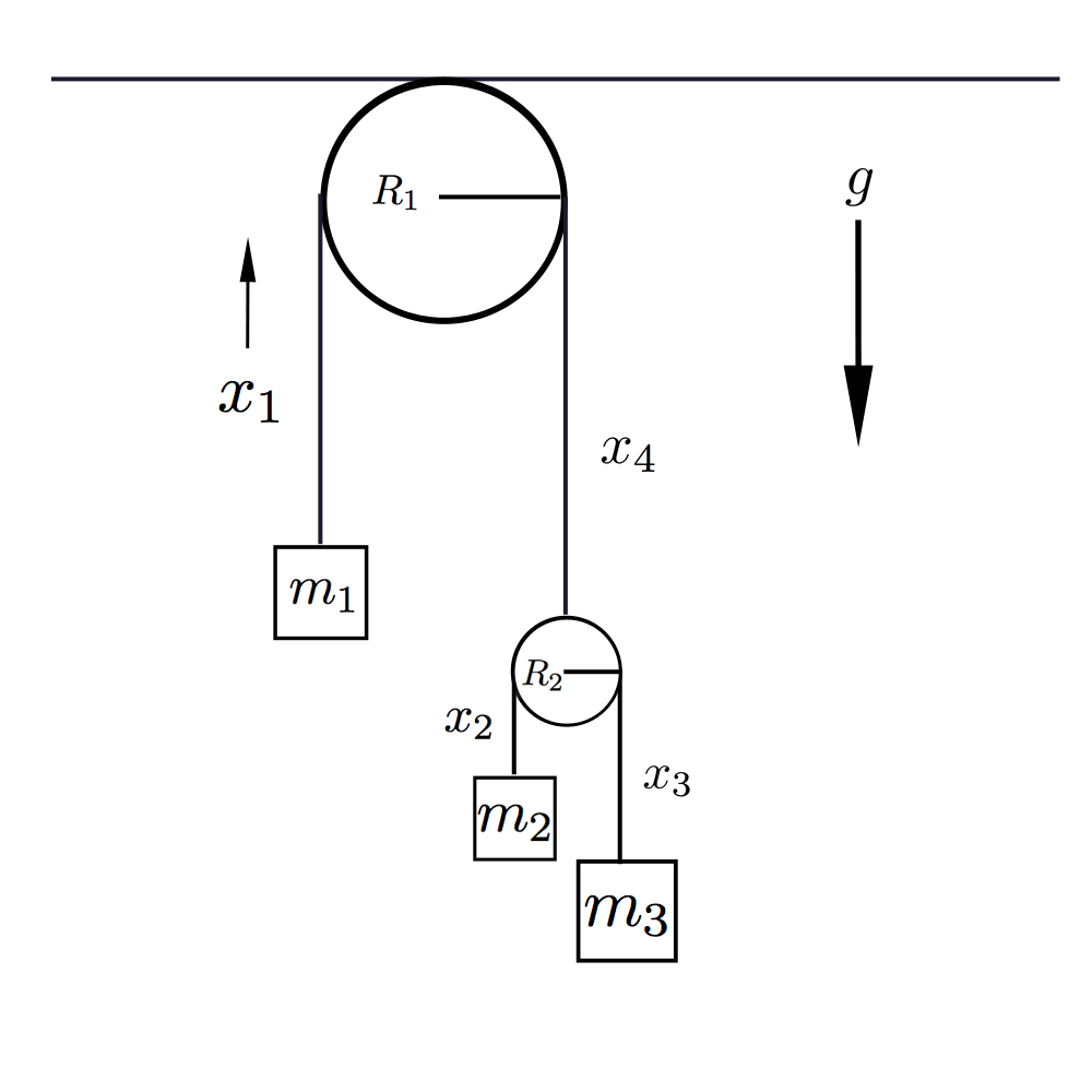
Figure 2: Double Atwood machine consisting of three masses, m1, m2, m3

Referring to Figure 2, we can let $x_{1}, x_{2}, x_{3}, x_{4}$ be the generalized coordinates of the system. $R_{1}$ will be the radius of the upper pulley, while $R_{2}$ is the radius of the lower pulley. If we define $l_{1}, l_{2}$ to be the lengths of the upper and lower strings, respectively, we may then write the coordinates $x_{2}, x_{4}$ in terms of $x_{1}$ and $x_{3}$ , and the constants $R_{1}, R_{2}, l_{1}, l_{2}$ :

$x_{4} = l_{1} - x_{1} - \pi R_{1}$ $x_{2} = l_{2} - x_{3} - \pi R_{2}$

Here, the $\pi R$ terms come from the length of string wrapped around the pulleys.

Now we may begin deriving the velocities associated with each mass. This will help to derive the kinetic energy of the system, for use with Lagrange’s equations.

For $m_{1}$ :

$v_{1} = \dot{x_{1}} \rightarrow v_{1}^{2} = \dot{x_{1}}^{2}$

For $m_{2}$ :

$v_{2} = \frac{d}{dt}(x_{4} + R_{2} + x_{2})$ $= \frac{d}{dt}(l_{1} - x_{1} - \pi R_{1} + R_{2} + l_{2} - x_{3} - \pi R_{2})$ $= -\dot{x_{1}} - \dot{x_{3}}$ $\rightarrow v_{2}^{2} = \dot{x_{1}}^{2} + 2\dot{x_{1}}\dot{x_{3}} + \dot{x_{3}}^{2}$

For $m_{3}$ :

$v_{3} = \frac{d}{dt}(x_{4} + R_{2} + x_{3})$ $= \frac{d}{dt} (l_{1} - x_{1} - \pi R_{1} + R_{2} + x_{3})$ $= \dot{x_{3}} - \dot{x_{1}}$ $\rightarrow v_{3}^{2} = \dot{x_{3}}^{2} - 2\dot{x_{1}}\dot{x_{3}} + \dot{x_{1}}^{2}$

Having each mass’s velocity squared, we may then write the systems total kinetic energy, T, as follows:

$T = \frac{1}{2}m_{1}v_{1}^{2} + \frac{1}{2}m_{2}v_{2}^{2} + \frac{1}{2}m_{3}v_{3}^{2}$ $= \frac{1}{2}m_{1}\dot{x_{1}}^{2} + \frac{1}{2}m_{2}(\dot{x_{3}}^{2} + 2\dot{x_{1}}\dot{x_{3}} + \dot{x_{1}}^{2}) + \frac{1}{2}m_{3}(\dot{x_{3}}^{2} - 2\dot{x_{1}}\dot{x_{3}} + \dot{x_{1}}^{2})$

Now, we need to determine the potential energy associated with each mass, in order to derive the system’s potential energy, U. We take the center of the upper pulley to be the origin.

For $m_{1}$ :

$U_{1} = -m_{1}gh$ $= -m_{1}gx_{1}$

For $m_{2}$ :

$U_{2} = -m_{2}gh$ $= -m_{2}g(R_{2} + l_{1} - x_{1} - \pi R_{1} + l_{2} - x_{3} - \pi R_{2})$

For $m_{3}$ :

$U_{3} = -m_{3}gh$ $= -m_{3}g(R_{2} + l_{1} - x_{1} - \pi R_{1} + x_{3})$

We may combine these to obtain the system’s potential energy:

$U = U_{1} + U_{2} + U_{3}$ $= -m_{1}gx_{1} - m_{2}g(R_{2} + l_{2} - x_{3} - \pi R_{2} + l_{1} - x_{1} - \pi R_{1}) - m_{3}g(R_{2} + x_{3} + l_{1} - x_{1} - \pi R_{1})$

Now we may establish the Lagrangian for the system. The Lagrangian is given as the difference between the kinetic and potential energies:

$\mathcal{L} = T - U$ $= \Big[\frac{1}{2}m_{1}\dot{x_{1}}^{2} + \frac{1}{2}m_{2}(\dot{x_{3}}^{2} + 2\dot{x_{1}}\dot{x_{3}} + \dot{x_{1}}^{2}) + \frac{1}{2}m_{3}(\dot{x_{3}}^{2} - 2\dot{x_{1}}\dot{x_{3}} + \dot{x_{1}}^{2})\Big] - \Big[-m_{1}gx_{1} - m_{2}g(R_{2} + l_{2} - x_{3} - \pi R_{2} + l_{1} - x_{1} - \pi R_{1}) - m_{3}g(R_{2} + x_{3} + l_{1} - x_{1} - \pi R_{1})\Big]$

We may now begin to determine the equation of motion for the masses. From Lagrange’s equations we have:

$\frac{\partial \mathcal{L}}{\partial x_{1}} - \frac{d}{dt}\frac{\partial \mathcal{L}}{\partial \dot{x_{1}}} = 0$ $(1)$

$\frac{\partial \mathcal{L}}{\partial x_{3}} - \frac{d}{dt}\frac{\partial \mathcal{L}}{\partial \dot{x_{3}}} = 0$ $(2)$

Working with the first equation we have:

$\frac{\partial \mathcal{L}}{\partial x_1} = (m_1 - m_2 - m_3)g$ $\frac{\partial \mathcal{L}}{\partial \dot{x_{1}}} = m_{1}\dot{x_{1}} + m_{2}\dot{x_{3}} + m_{2}\dot{x_{1}} - m_{3}\dot{x_{3}} + m_{3}\dot{x_{1}}$ $= (m_{1} + m_{2} + m_{3})\dot{x_{1}} + (m_{2} - m_{3})\dot{x_{3}}$ $\rightarrow \frac{d}{dt}\frac{\partial \mathcal{L}}{\partial \dot{x_{1}}} = (m_{1} + m_{2} + m_{3})\ddot{x_{1}} + (m_{2} - m_{3})\ddot{x_{3}}$

Putting these pieces together gives:

$(m_{1} - m_{2} - m_{3})g = (m_{1} + m_{2} + m_{3})\ddot{x_{1}} + (m_{2} - m_{3})\ddot{x_{3}}$ $(3)$

Working with equation $(2)$ , we obtain:

$\frac{\partial \mathcal{L}}{\partial x_{3}} = (m_{3} - m_{2})g$ $\frac{\partial \mathcal{L}}{\partial \dot{x_{3}}} = (m_{2} - m_{3})\dot{x_{1}} + (m_{3} + m_{2})\dot{x_{3}}$ $\rightarrow \frac{d}{dt}\frac{\partial \mathcal{L}}{\partial \dot{x_{3}}} = (m_{2} - m_{3})\ddot{x_{1}} + (m_{3} + m_{2})\ddot{x_{3}}$

Putting these pieces together gives:

$(m_{3} - m_{2})g = (m_{2} - m_{3})\ddot{x_{1}} + (m_{3} + m_{2})\ddot{x_{3}}$ $\rightarrow \ddot{x_{3}} = \frac{1}{(m_{2} + m_{3})}\big[(m_{3} - m_{2})g - (m_{2} - m_{3})\ddot{x_{1}}\big]$

We may now plug this result into equation (3):

$(m_{1} - m_{2} - m_{3})g = (m_{1} + m_{2} + m_{3})\ddot{x_{1}} + \frac{(m_{2} - m_{3})}{(m_{2} + m_{3})}\big[(m_{3} - m_{2})g - (m_{2} - m_{3})\ddot{x_{1}}\big]$ $\rightarrow \big[(m_{2} + m_{3})(m_{1} - m_{2} - m_{3}) - (m_{2} - m_{3})(m_{3} - m_{2})\big]g = \big[(m_{2} + m_{3})(m_{1} + m_{2} + m_{3}) - (m_{2} - m_{3})^{2}\big]\ddot{x_{1}}$

$\rightarrow (-4m_{2}m_{3} + m_{1}m_{2} + m_{1}m_{3})g = (4m_{2}m_{3} + m_{1}m_{2} + m_{1}m_{3})\ddot{x_{1}}$
$\boxed{\ddot{x_1} = \Bigg[\frac{-4m_{2}m_{3} + m_{1}m_{2} + m_{1}m_{3}}{4m_{2}m_{3} + m_{1}m_{2} + m_{1}m_{3}}\Bigg]g}$

Plugging this back into the expression for $\ddot{x_{3}}$ we find:

$\boxed{\ddot{x_{3}} = \frac{(m_{3} - m_{2})}{(m_{2} + m_{3})}g\Bigg[1 - \frac{4m_{2}m_{3} - m_{1}m_{2} - m_{1}m_{3}}{4m_{2}m_{3} + m_{1}m_{2} + m_{1}m_{3}}\Bigg]}$

For fun, we may substitute values in for $m_{1}$ , $m_{2}$ , and $m_{3}$ . Let $m_{1} = 4m$ , $m_{2} = m$ , and $m_{3} = 3m$ . Then we find:

$\ddot{x_{1}} = \Bigg[\frac{-4(3m^{2}) + 4m^{2} + 12m^{2}}{4(3m^{2}) + 4m^{2} + 12m^{2}}\Bigg]g$ $= \frac{g}{7}$ $\ddot{x_{3}} = \frac{1}{(m_{2} + m_{3})}\big[(m_{3} - m_{2})g - (m_{2} - m_{3})\frac{g}{7}\big]$ $= \frac{4g}{7}$

In addition, we may plug in proper values for the masses. Let $m_{1} = 500g$ , $m_{2} = 200g$ , and $m_{3} = 400g$ . Then we have:

$\ddot{x_{1}} = \frac{-4(80000) + 100000 + 200000}{4(80000) + 100000 + 200000}g$ $= \frac{-g}{31}$ $\ddot{x_{3}} = \frac{1}{600}\big[200g+200\big(\frac{-g}{31}\big)\big]$ $= \frac{10g}{31}$

Note that in each case, the units work out and we are left with accelerations with the proper units.

Notes:

String tends to slip off of pulleys if pulled too quickly.

Written by Madison Harris