Coupled Pendulum | UCSC Physics Demonstration Room

Demo:

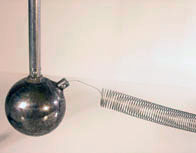
Two identical pendulums are attached by a soft spring and exchange energy with each other. This demonstration is useful for elementary physics, mechanics, and particle physics. The instructor can show the audience normal modes with or without the spring.

Explanation:

The math and physics used to describe the motion of the double pendulum are somewhat complicated and more suited to upper division physics students than students enrolled in introductory physics. That being said, this is a good demo to show students of all abilities if you are not expecting to go through all of the derivations.

This explanation is divided into three parts. The first part is a general explanation of why we use the math that we use, and how it relates to the demo and the effects that we see. The second part is a derivation of the two normal modes of the system, as modeled by two masses attached to a spring without the pendulum aspect. The third part adds in the swinging motion from the pendulum and the potential energy held by the suspended pendulums, using a Lagrangian derivation for the equations of motion.

Some initial assumptions about the nature of the pendulum are:

The two pendulums are identical and have the same natural frequency when not attached by a spring
The pendulums are “simple” (i.e. they are attached to massless rods and the weights are point particles at the ends)
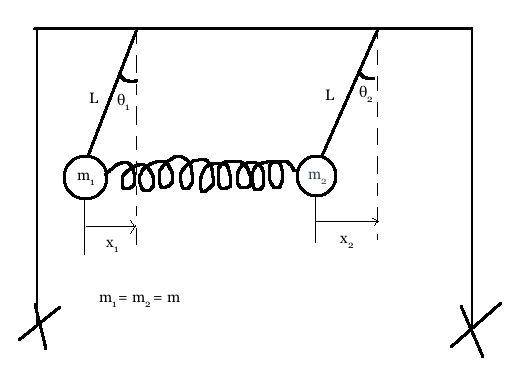
Angles of deflection of masses 1 and 2 are θ₁, θ₂ (measured from the vertical) and are small such that $sin\theta \approx \theta$ , $cos\theta \approx 1 - \cfrac{\theta^2}{2}$
The spring constant = K, the length of each of the rods = L, and the masses m₁ = m₂ = m

coupledpendulum

Part One:

When you pull on mass 1 and let it go, it will pull on mass 2 because they are connected by the spring. This generates a force on mass 2 that changes with the frequency of mass 1’s motion. As mass 1 loses energy, mass 2 will have an energy increase that is exactly the same as the energy lost by mass 1. This is because (ideally) this is a closed system that does not lose any energy to its surroundings or to friction. As the energy in a pendulum increases and decreases, its amplitude will increase and decrease, respectively. This means that as mass 1’s amplitude (x₁) decreases, mass 2’s amplitude (x₂) will increase. Eventually mass 1 will lose all its energy to mass 2, and its amplitude will go to zero. At that point, mass 2 begins losing energy to mass 1, and the cycle repeats.

How do we explain the motion of this double pendulum? What we see resembles the same pattern we see with beat frequencies, when you overlap wave equations with slightly different frequencies.

Source

As you can see above, the black and red waves have slightly different frequencies. The sum of the two waves will be the largest when they are in phase (when one crest aligns with another crest), and when they are out of phase (when one crest aligns with a trough), the wave will cancel out. When the amplitudes of the two waves are the same, the amplitude when the two are in phase will be twice the height of either component wave, and when the two are out of phase the amplitude will be zero.

We see similar motion displayed in the double pendulum. Each mass has its own beat frequency that cycles from a large amplitude to zero amplitude and back. One mass will have the highest amplitude when the other mass has an amplitude of zero. This means that the motion of the masses are governed by the sum of two independent wave functions.

It is fairly easy to see the two frequencies of this system that govern the total motion. All we have to look for are the two forms of motion (modes) where both pendulums move constantly with one motion and do not change cyclically. It is at these points where the one wave function is zero, such that the other is the only one acting on the system, and therefore, the only one that is seen.

The first is if we displace the two masses with the exact same value in the same direction (both x₁ and x₂ to the left or right). Because the masses are equal and the length and k of the springs are equal, both masses will move exactly the same, swinging back and forth equally, never losing energy to one or the other. The second mode is if you displace masses 1 and 2 in an equal and opposite way (if you displaced mass 1 to the left, you would displace mass 2 to the right with an equal length of displacement, x₂ ). In this case, because the masses will move in equal and opposite directions, there will be a node at the center of the spring that has a displacement of zero.

It is important here to note that the reason we get the beat frequencies is because the first and second modes are of slightly different frequencies. The mode of the second mass will correspond to a slightly higher frequency due to the restoring force from the spring acting on it.

In summary, there are two equations of motion that govern this system of pendulums, one with a mode where both masses are moving in the same direction and the other where the pendulums are moving in the exact opposite direction. The combination of these two modes makes up every possible beat frequency and amplitude of the system¹.

Part Two:

This equation will give the eigenvectors a and b that describe the ways that the two pendulums move with respect to one another (the modes of the system). The way to find the eigenfrequencies of the system is with this equation:

$latex det([K]-ω²[M]) = 0

for the values of ω, and then use these values to find the eigenvector a and b that describe the motion of the system. In this equation, matrix K is the “stiffness matrix” of the spring and matrix M is the “mass matrix”. This is the equation used to find the eigenfrequencies and eigenvectors of the system.

The matrix [K] can be found by taking the partial derivatives of the potential energy equation, and the matrix [M] is just the mass (m) of the pendulums in positions M₁₁ and M₂₂.

$U = \cfrac{1}{2} k (x_2 - x_1)^2$

$= \cfrac{1}{2}kx_2^2 + \cfrac{1}{2}kx_1^2 - kx_1x_2$

$K = \left[\begin{array}{cc}K_{11} &K_{12}\\ K_{21}&K_{22}\end{array}\right]$

$K_{11} = \cfrac{\partial ^2 U}{\partial x_1} = k$

$K_{12} = K_{21} = \cfrac{\partial ^2 U}{\partial x_1 x_2} = -k$

$K_{22} = \cfrac{\partial ^2 U}{\partial x_2} = k$

$K = \left[\begin{array}{cc}k &-k\\ -k &k\end{array}\right]$

$M = \left[\begin{array}{cc}M_{11} &M_{12}\\ M_{21}&M_{22}\end{array}\right]$

$M_{11} = m$

$M_{12} = M_{21} = 0$

$M_{22} = m$

$M = \left[\begin{array}{cc}m &0\\ 0&m\end{array}\right]$

Once you have the K and M matrices you can solve the characteristic equation to solve for ω:

$det[K-\omega ^2 M] = 0$

$det\left[\begin{array}{cc}k-\omega ^2m &-k\\ -k&k- \omega ^2m\end{array}\right] = 0$

$(k-\omega ^2m)^2 - (-k)^2 = 0$

$(k-\omega ^2m)^2 = k^2$

$k-\omega^2m = \pm k$

$\swarrow$ $\searrow$

$k-\omega_1^2m = k$ $k-\omega_2^2m = -k$

$-\omega_1^2m = 0$ $\omega_2^2m = 2k$

$\boxed{\omega_1 = 0}$ $\boxed{\omega_2 = \sqrt{\cfrac{2k}{m}}}$

Once you have the values of ω₁ and ω₂ you can use those to find the eigenvectors of the system (a and b), which show the relative motions of the pendulums.

$\textcircled{1} \omega_1 = 0$ $\textcircled{2} \omega_2 = \sqrt{\cfrac{2k}{m}}$

$(-k)a_{1} + ka_{2} = 0$ $(k-\cfrac{2k}{m}(m))b_{1} + (-k - \cfrac{2k}{m}(0))b_2 = 0$

$a_2 = a_1 \: \: \: \: \: \: \: \: \: \: \: \: \: \: \: \: \: \: \: \: \: \: \: \: \: \: \: \: \: \: \: \: \: \: \: \: \: \: \: \: \: \: \: \: \: \: \: \: \: \: \: \: \: \: \: \: \: \: \: \: \: \: \: \: (-k)b_1 - kb_2 = 0$

$b_1 = -b_2$

$a =\left[\begin{array}{c}1\\ 1\end{array}\right]$ $b =\left[\begin{array}{c}-1\\1\end{array}\right]$

These two results tell us that the two modes of motion for the coupled pendulum are when the pendulums are both swinging in the same direction (matrix a) and when the pendulums are swinging in opposite directions (matrix b).

In addition to finding the modes of the system, we can also find the eigenfrequencies specific to this system by using the Lagrange method of derivation.

This system has two degrees of freedom, where θ₁ and θ₂ are the independent variables. The number of degrees of freedom that a system has is the number of independently variable factors which affect the range of states that the system can be in. If we had a system with just one pendulum we would have just one degree of freedom, θ.

This demo is good to show how each pendulum can affect the frequency and the amplitude of the other pendulum. Typically what happens when one of the pendulums is swung is that it begin with a large amplitude, and some of the energy that is contained within the first pendulum is transferred to the second through the spring. The second pendulum will begin to swing as well, slowly increasing its amplitude as the amplitude of the first pendulum decreases. As soon as the first pendulum stops swinging, the cycle will repeat and it will begin to take energy from the second pendulum and will begin to swing with a greater and greater amplitude. They will go in this pattern, with one pendulum “taking” energy from the other until all of the energy in the system is lost to friction and air resistance and both the pendulums stop swinging.

Part Three:

Following is the derivation of the eigenfrequencies of the system using the Lagrange method:

First we have to find the kinetic energy (T) and potential energy (U) of the system as a whole:

$T = \cfrac{1}{2}m(\dot{x}_1^2 + \dot{x}_2^2)$

$U = mg(y_1 + y_2) + \cfrac{1}{2}k(x_2 - x_1)^2$

$= \cfrac{mg}{2l}(x_1^2 + x_2^2) + \cfrac{1}{2}k(x_2 - x_1)^2$

To get T we use the kinetic energy equation $T = \cfrac{1}{2}mv^2$ . We know that $v=\dot{x}$ and we can add T for both mass one and two together to give us the above equation.

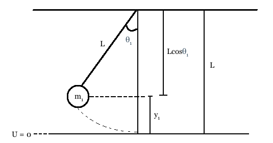
To get the potential energy we have to add up potential energy from two different sources: The potential energy of the masses because their vertical position changes during their motion and the potential energy contained within the spring. The gravitational potential energy contained in the system from the two suspended masses gives a first term equal of $U = mgh$ (for masses one and two). The gravitational potential energy can be calculated from anywhere, so we define the “zero” of the potential energy to be from where the masses are on the y axis when θ=0. This is the point of equilibrium in the system and is where the pendulums hang straight down from their support beam. This gives the gravitational potential energy of the system $U_1 = mg(y_1 + y_2)$ .

The second potential energy term we get from the potential energy contained within the spring connecting the two masses. Potential energy from a spring is $U=\frac{1}{2}kx^2$ where x is the displacement of the spring in the positive or negative direction from its equilibrium point, where it will naturally be if no net force is exerted on it. We can tell that the total displacement from equilibrium of our spring is equal to the displacement of mass 2 (x₂) minus the displacement of mass 1 (x₁). This makes the equation for potential energy contained in the spring: $U_2 = \cfrac{1}{2}k(x_2 - x_1)^2$ .

The total potential energy in the system is therefore:

$U_1 + U_2 = U = mg(y_1 + y_2) + \cfrac{1}{2}k(x_2 - x_1)^2$

The next step in finding the eigenfrequencies for the system is to figure out the equations of constraint that relate x to y so that we can make the Lagrangian. We relate y to x as follows:

$y_1 = l-lcos\theta_1$

$\approx l-l(1-\cfrac{\theta_1^2}{2})$

$\approx \cfrac{l}{2}\theta_1^2 \approx \cfrac{l}{2}(\cfrac{x_1}{l})^2$

$\approx \cfrac{x_1^2}{2l}$

This approximation can be made for both x₁ and x₂. We used the small angle approximation for cosθ to the second order (taking it to the first order may give us a trivial solution). This second order approximation gives us $\cfrac{l}{2}\theta_1^2$ . We know that small $\theta \approx \frac{x}{l}$ which gives us the last term of our approximation. Using these approximations we can relate y, θ, x₁ and x₂ to two generalized coordinates, $X$ and $x$ :

$x = x_2 - x_1$ $\dot{x} = \dot{x_2} - \dot{x_1}$

$X = x_2 + x_1$ $\dot{X} = \dot{x_2} + \dot{x_1}$

$x_2 = \cfrac{x + X}{2}$ $x_1 = \cfrac{X - x}{2}$

$\dot{x_2} = \cfrac{\dot{x} + \dot{X}}{2}$ $\dot{x_1} = \cfrac{\dot{X} - \dot{x}}{2}$

Now we can write T and U in terms of generalized coordinates $X$ and $x$ :

$T = \cfrac{1}{2}m\big[(\cfrac{\dot{X} - \dot{x}}{2})^2 + (\cfrac{\dot{X} - \dot{x}}{2})^2\big] = \cfrac{1}{4}m[\dot{X}^2 + \dot{x}^2]$

$U = \cfrac{mg}{4l}[X^2 + x^2] + \cfrac{1}{2}kx^2$

$L = T - U$

$L = \cfrac{1}{4}m[\dot{X}^2 + \dot{x}^2] - \cfrac{mg}{4l}[X^2 + x^2] - \cfrac{1}{2}kx^2$

Once we have the Lagrangian constructed, all we need to do is take the appropriate derivatives:

$\textcircled{1} \cfrac{\partial L}{\partial X} = \cfrac{d}{dt}\cfrac{\partial L}{\partial \dot{X}}$ $\textcircled{2} \cfrac{\partial L}{\partial x} = \cfrac{d}{dt}\cfrac{\partial L}{\partial \dot{x}}$

$-\cfrac{mg}{2l}X = \cfrac{1}{2}m\ddot{X}$ $-(\cfrac{mg}{2l} + k)x = \cfrac{1}{2}m\ddot{x}$

$\ddot{X} = -\cfrac{g}{l}X$ $\ddot{x} = -(\cfrac{g}{l} + \cfrac{2k}{m}x)$

$\boxed{\omega_1 = \sqrt{\cfrac{g}{l}}}$ $\boxed{\omega_2 = \sqrt{\cfrac{g}{l} + \cfrac{2k}{m}}}$

This gives us the eigenfrequencies (ω₁ and ω₂). The mass will thus oscillate at frequencies that are linear combinations of ω₁ and ω₂. These will depend on the rod length, spring constant, mass m, and gravity.

Note: To release the spring use the screwdriver attached to the frame.

Written by: Sophia Sholtz

Lagrange derivation by Steve Martin

Richard Feynman’s description of Normal Modes in Volume 1, chapter 48, section 7 of Feynman’s Lectures on Physics