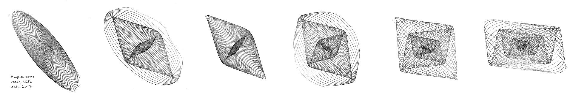
Harmonograph | UCSC Physics Demonstration Room

A harmonograph is a simple mechanical machine consisting of multiple pendulums and is used to demonstrate the effects of coupled oscillators by tracing out geometric patterns. Our harmonograph consists of two pendulums and traces Lissajous Figures when set in motion.

Equipment:

Harmonograph apparatus
Paper (a stack of paper works better for smoother lines)
Pen (Pilot Easytouch pen works best)
Clips to hold paper on drawing table

Demo:

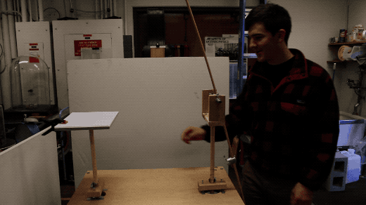
Begin by placing a clean sheet of paper on the drawing table. Make sure the pen arm is raised, and set both pendulums in action. While the pendulums are moving, gently lower the pen arm to make contact with the paper. (Click to view GIF).

Explanation:

Pendulums exhibit simple harmonic motion which is governed by the following equation:

$x(t) = Asin(\omega t + \delta)e^{-dt}$

$A$ is the amplitude of the pendulum, $\omega$ is the frequency, and $\delta$ is phase. The exponential term represents the damping of the pendulum, with $d$ acting as the damping coefficient.

For our harmonograph, the two pendulums are governed by similar equations:

$x(t) = Asin(\omega_{1} t + \delta_{1})e^{-d_{1}t}$ ,

$y(t) = Bsin(\omega_{2} t + \delta_{2})e^{-d_{2}t}$

When the pendulums are set in motion, the resulting image is a compilation of $x(t)$ vs. $y(t)$ . Since the two pendulums are perpendicular, the resulting image represents Lissajous Figures.

We may change the frequencies $\omega_{1}$ and $\omega_{2}$ in order to get different images. Frequency is related to length through the following formula:

$\omega = \sqrt{g/l}$

Thus, if we change the length of the pendulums, we can change the frequency to generate different images. To do so, simply move the weights on the pendulums up and down as desired.

A GIF of Python simulated motion is shown below (click to view GIF).

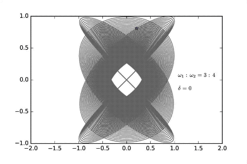
A Python produced simulated video is also available.

For those interested in a more detailed derivation of how our harmonograph was built/how it works see below.

Derivation of Frequency Relations:

Due to the substantial weight of the drawing platform and pen assembly, our harmonograph does not consist of two simple pendulums. As such, we need to account for the mass of each of the top components when determining frequency. The following is a derivation of the angular frequency for a pendulum consisting of two bobs.

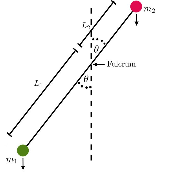
To begin, we determine the torque around the fulcrum. This is given by:

$\tau = I \alpha = \vec{F} \times \vec{r}$ .

We know that:

$\vec{F} \times \vec{r} = Frsin\theta$

Then, assuming the same angular displacement for both the upper and lower pendulums, we have the following relationships for the torque on each bob:

$\tau_{1} = -m_{1}gL_{1}sin\theta$ ,

$\tau_{2} = m_{2}gL_{2}sin\theta$

These combine to give a total torque of:

$\tau_{tot} = gsin\theta(m_{2}L_{2} - m_{1}L_{1})$

But we also know that:

$I\alpha = (m_{1}L_{1}^{2} + m_{2}L_{2}^{2})\ddot{\theta}$

Thus we may equate the two relationships to obtain:

$\ddot{\theta} - gsin\theta\frac{(m_{2}L_{2} - m_{1}L_{1})}{(m_{1}L_{1}^{2} + m_{2}L_{2}^{2})} = 0$

Then, assuming small angle displacements, we have the characteristic frequency:

$\omega_{0}^{2} = \ddot{\theta} = \frac{(m_{2}L_{2} - m_{1}L_{1})}{(m_{1}L_{1}^{2} + m_{2}L_{2}^{2})}$

We may now derive the relationships between bottom pendulum masses that are needed to obtain various Lissajous figures. For the platform assembly we have:

$\omega_{p}^{2} = g\frac{|m_{tp}L_{tp} - m_{bp}L_{bp}|}{m_{tp}L_{tp}^{2} + m_{bp}L_{bp}^{2}}$

The mass of the platform assembly is denoted by $m_{tp}$ and the length of the top pendulum is denoted by $L_{tp}$ . Similarly, the mass on the bottom of the pendulum is denoted by $m_{bp}$ while the bottom length is $L_{bp}$ . For the pen holder assembly we have:

$\omega_{e}^{2} = g\frac{|m_{te}L_{te} - m_{be}L_{be}|}{m_{te}L_{te}^{2} + m_{be}L_{be}^{2}}$

Here the mass of the pen assembly is marked as $m_{te}$ , the top length by $L_{te}$ , the bottom quantities are denoted by $m_{be}$ and $L_{be}$ .

We want to define a relationship between $m_{bp}$ and $m_{be}$ such that we can create common ratios of frequencies (i.e. $\omega_{p}/\omega_{e}$ ).

To keep calculations less messy, let’s define the following constants:

$\alpha = m_{tp}L_{tp}$ ,

$\beta = m_{tp}L_{tp}^{2}$ ,

$\gamma = m_{te}L_{te}^{2}$ ,

$\lambda = m_{te}L_{te}$ ,

$\mu =\frac{\omega_{p}^{2}}{\omega_{e}^{2}}$

If we choose to let $L_{tp} = L_{te} = L$ , we may rewrite a relationship for $\frac{\omega_{p}^{2}}{\omega_{e}^{2}}$ as follows:

$\mu = \frac{(\alpha - m_{bp}L)}{(\beta + m_{bp}L^{2})}\frac{(\gamma + m_{be}L^{2})}{(\lambda - m_{be}L)}$ .

Solving for $m_{bp}$ gives:

$m_{bp} = \frac{(\alpha \gamma - \mu \beta \lambda) + m_{be}(\alpha L^{2} + \mu \beta L)}{m_{be}L^{3}(1-\mu ) + (\gamma L + \mu \lambda L^{2})}$

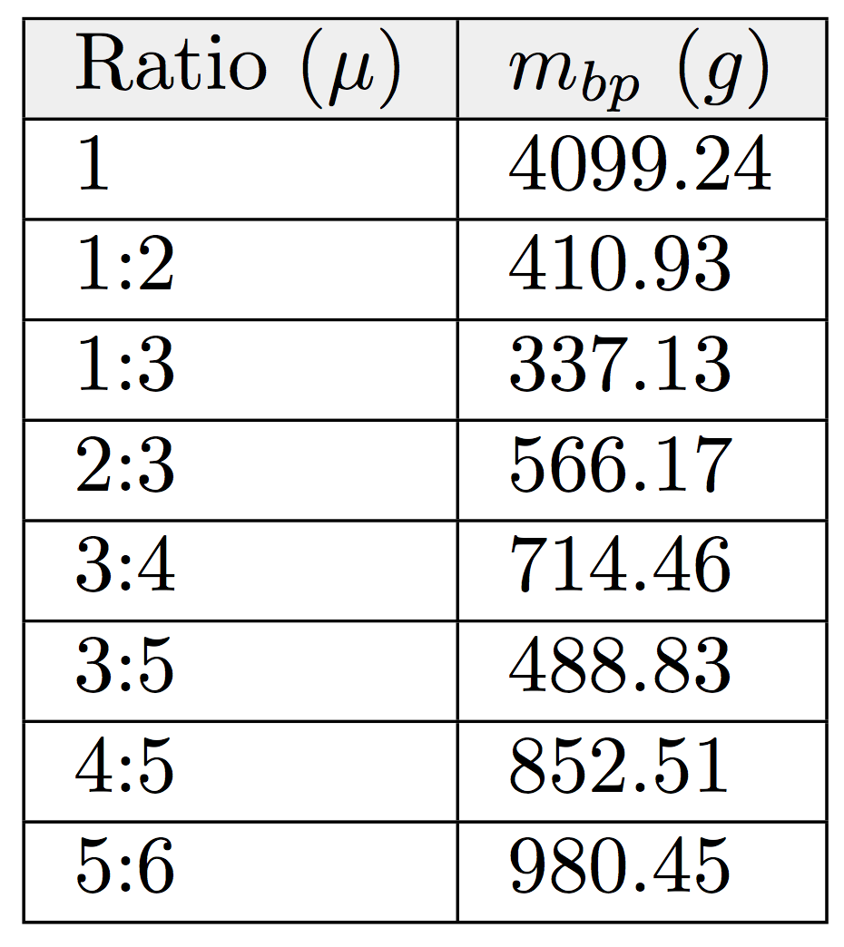
The values of the arbitrary constants are known, and we can set $m_{be}$ to an arbitrary weight (we only care about the ratios of quantities). Doing so, we are able to find the various platform weights that are need to generate Lissajous figures. These are shown in the table below.

How the UCSC Harmonograph Was Built:

The UCSC harmonograph consists of two pendulums, suspended above a wooden table, that move in perpendicular directions. One pendulum consists of a drawing table on top, the other consists of a support arm to hold a pen. The drawing platform is a simple plank of wood connected to a bowl using a laboratory collar to connect the two pieces together. The pen apparatus consists of a U-shaped cage that contains a narrow piece of threaded steel. A narrow dowel is perpendicularly connected to the steel rod and reaches towards the drawing table. This is attached to a pen. The pendulums are supported by wooden crossbeams that contain two sharp nails which act as pivots and allow them to oscillate (see Figure 1, click to view GIF).

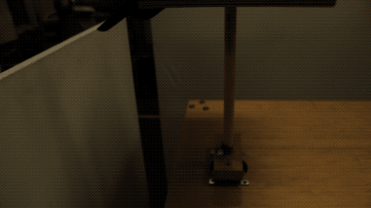
Figure 1

Written by Madison Harris